Surface gradients cannot be defined for categorical data, so wombling procedures developed for numeric data do not apply. For this situation, Oden et al. (1993) developed categorical wombling. Categorical wombling is available for point and polygon datasets. For raster datasets, it is only available for datasets imported in Grid ASCII format.
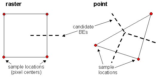
Categorical wombling uses dissimilarity metrics for Boundary Likelihood Values (BLVs), calculated between pairs of adjacent sampling locations. The dissimilarity values are used to evaluate candidate Boundary Elements (cBEs). For categorical wombling on raster and point data, candidate Boundary Elements (cBEs) are the lines equidistant from the sample locations (see figure below). For categorical polygon data, the cBEs are the edges of the original polygons (see polygon wombling). cBEs only become boundaries when the BLVs are above the user threshold. BoundarySeer connects Boundary Elements (BEs) into subboundaries if they are adjacent.
Categorical dissimilarity metrics include taxonomic, genetic and mismatch distances (Johnson and Wichern 1982), and in practice are selected to reflect the nature of the variables in the analysis. BoundarySeer currently includes only mismatch distance, but future versions will include other metrics, as well as an editor that will allow users to input their own custom metrics.
Fuzzy categorical wombling is meaningful only on data sets with more than one variable. Mismatch values for individual variables are binary (two values are the same or they are mismatched). Therefore, even if you specify a fuzzy boundary, the BLVs will be either 0 or 1 for univariate data sets. Thus, you will not detect any intermediate BLVs, and intermediate values are necessary for a gradation in boundary membership. For multivariate data sets, BLVs will be the average of mismatch values for each individual variable, so a range of BLVs (and therefore fuzzy BMVs) is more possible.
Barbujani et al. (1990) supplemented their findings from lattice (here called raster) wombling by applying a form of categorical wombling to their Eurasian genetic data. They calculated the genetic distance between samples, and then scaled this distance by the geographic distance between the locations. Oden et al. (1993) used a mismatch metric and multivariate linguistic data to quantify language boundaries in Europe. These boundaries identified contact zones between areas where different languages were spoken, and confirmed the large-scale dialectical groupings generally accepted by linguists. Fortin and Drapeau (1995) used a metric defined as 1 minus the match coefficient (Legendre and Legendre 1983) and tree presence/absence data to identify boundaries in species turnover in a Quebec hardwood forest.
See also: