


Implementation of Spatial Regression
The Spatial regression method in SpaceStat has three types of regression: Ordinary Least Squares, Spatial lag and Spatial Error.
Ordinary Least Squares (OLS)
The implementation of OLS is no different from Aspatial Linear Regression and your parameter estimates will be the same after running the same model in either method.
The difference between these two options is that the OLS method will also run diagnostics which test some of the usual assumptions of OLS (heteroskedascity, non-normality, etc). The diagnostics will also use a spatial weight set to assess whether or not a spatial component would improve the results of the model.
Spatial Lag
The spatial lag model assumes that the dependent variable at a particular location is not only explained by the independent variables in the model but also by the values of the dependent variable itself at neighboring locations. The regression model is in matrix form (for NT observations)
y = rW1y + Xb + e
Here y denotes the dependent variable matrix, X denotes a matrix of independent variable observations, b denotes the regression coefficients and the error terms e are normally distributed with zero mean and variance s2. The coupling to neighboring values of the dependent variable takes place through the spatial weights matrix W1 (which are usually row-standardized) and is modulated via the lag parameter r.
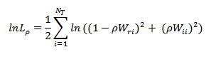
The log-likelihood can be written
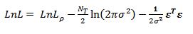
where the first two terms denote the normalization contributions that depend on the trace of the logs of the weight matrices and the last term (corresponding to a sum of squares) contains mixtures of residuals, weight matrices and regression coefficients e = Ay - Xb with the lag term written A = 1 - rW1.
Minimizing the log-likelihood with respect to the elements of b determines the regression coefficients as b = (XTX)-1XTAy with the predicted values of the dependent variable given by E(y) = A-1Xb. The remaining parameters are determined by substituting the regression coefficients back into the log-likelihood and using a bisection search to find the optimal value of the lag parameter. Lastly we require the eigenvalues of the spatial weights matrix for the normalization contribution
For spatial error the model appears the same as for OLS or aspatial regression
y = Xb + e
but assumes that correlations between the errors e at neighboring observations can be specified by the spatial weights matrix modulated by a spatial error coefficient l, namely e = lW2 e + m where W2 denotes the spatial weights matrix and the remaining errors m have variance s2. The rest of the notation is the same as in the spatial lag case.
The log-likelihood can be written
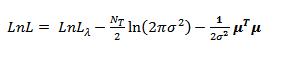
where the spatial weights normalization component is
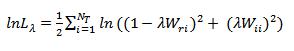
again expressed in terms of the eigen-values of the spatial weights matrix.
Writing the error terms in the form m = Be where B = 1 - lW2 we can obtain the regression coefficients from minimizing the log-likelihood as b = (XTBTBX)-1XTBTBy which has the form expected from a generalized least squares treatment. Substituting this back into the log-likelihood leads to an expression that can be minimized using a bisection search to locate the optimal value of the spatial error parameter l.