Implementation of Linear Regression in SpaceStat

In SpaceStat, a program designed for analysis of space-time datasets, we have implemented aspatial forms of regression as special cases of geographically weighted regression; the case where the neighborhood includes all of the locations in your focal geography.  This linkage with geographically-weighted regression means that SpaceStat retains weighting options for aspatial linear regression, although these weight values no longer have any functional dependence on location (spatial neighborhood).  Examples of when you might choose to use a weighting function in aspatial regression are described here.  We'll start the description of how regression is implemented with the general equation we have used to represent aspatial linear regression models, and then review the approach SpaceStat uses to obtain parameter estimates, sums of squares, R-squared, and p-values.  

Obtaining the parameter estimates

SpaceStat computes parameter estimates for linear regression using a maximum likelihood approach.  Used in this context, "likelihood" refers to the probability that the dependent variable can be predicted from the independent variable(s).  Given the probability function for a single observation, we can write the joint probability function (likelihood function) as a product of the individual probabilities.  In the following equations, the brackets around the beta, which symbolizes the regression coefficients, indicates that we are estimating two or more regression coefficients.

 

Next, we need to define the probability function for the individual observations (on the right side of our equation above), which is shown below.  For linear regression, probability densities are normally distributed (Gaussian), with a zero mean for the residuals and a variance which can differ between observations (note the "i" subscript for the variance components of the equation).  Recall that the symbol (pi), represents a constant (approximately 3.14).  

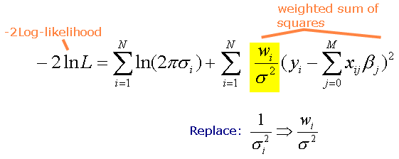
To estimate parameter values, we use -2 times the logarithm of the Likelihood, because this form has properties that facilitate the likelihood estimation process.  In addition to making this change, we also change how the variance is expressed to allow the incorporation of weights.  Recall we are focused here on aspatial regression, but the formulation here parallels that for geographically weighted regression, and can accommodate non-spatial weights.  The variance in the equation above can vary by observation; in the equation below, we have replaced the original variance expression with one that includes a constant variance and a weighting factor that varies by observation (see highlighted part of the equation).  Thus, we can now think of the non-constant variance as being equivalent to a weighting factor that varies by observation times a constant variance.

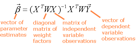
To solve for the regression coefficients (parameter estimates), SpaceStat finds values for these coefficients that minimize the weighted sum of squares.  The actual computation of the parameter estimates involves operations on a suite of matrices and vectors, and is summarized below.  Note that X with the superscript "T" refers to the transposed X matrix.   

Referring back to the regression equation above, the independent variable observation matrix X is regarded as a fixed quantity linking the random error (assumed to have a mean of 0 and a variance ) with the observed values of the dependent variable Y, and with the regression coefficients.  Hence, the mean value and standard error of the regression parameters can be obtained in terms of the regression parameters themselves, the inverse of the combination (XTWX)-1 and the error variance .  The expected value of the dependent variable at each location comes from the product of the independent variable matrix and the vector of the least squares regression coefficients.  These expected values of y are then used to calculate the residual sum of squares and total sum of squares (see below).  

Evaluating the model:  Calculating sums of squares

As described above, after obtaining the parameter estimates, SpaceStat calculates the estimated mean, standard error, and residual error for the dependent variable (y) at each observation.  These values are then used to calculate the residual sum of squares (RSS) and the total sum of squares (TSS) using the formulas below.  Recall that "N" is the number of observations, and "M" is the number of independent variables. In the TSS formula, the y-bar term represents the mean value of the dependent variable observations.  

Model R-squared and adjusted R-squared values

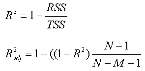
The residual sum of squares and the total sum of squares are used to calculate the model R-squared value, an overall measure of the strength of the association between the model developed using the independent variables, and the observed values of the dependent variable y.  Along with R-squared, SpaceStat also reports an adjusted R-squared value.  The adjusted R-square is a measure of model fit that allows you to compare across models with the same dependent variable using different numbers of independent variables.  The adjustment involves multiplying the R-squared value by the ratio of the number of observations, N, divided by N-M (1 is subtracted from both, as shown below).  As the number of observations increases, especially for models with a small number of predictor variables, the difference between the R-squared and adjusted R-squared values will approach zero.

Significance of the regression model

The significance of the overall model is assessed by calculating the F-value (see formula below), and then comparing that test statistic to values from an F distribution.  Higher F-values are associated with lower p-values.  In other words, if your independent variables explain a large proportion of the variance in your dependent variable (i.e., small residual variance), your calculated F-value will be high, and will be associated with a low probability of having attained this F-value by chance.  The p-value reported by SpaceStat should then be compared to your pre-set alpha level (typically 0.05).  If the p-value is smaller than your alpha, you can conclude that your model provides reliable predictions of the dependent variable.  However, if your model includes more than one independent variable, this result does not help you to understand the relative importance of each in making reliable predictions.

The ANOVA table  

In addition to reporting the significance of the model as a whole, SpaceStat also uses an Analysis of Variance (ANOVA) approach to evaluate the importance of individual terms within the regression model.  Specifically, SpaceStat calculates the Type III (Marginal) Sum of Squares.   The Type III sum of squares for a term in the model equals the residual sum of squares (RSS) for the full model without that term minus the RSS for the full model, divided by the degrees of freedom for that term to get the Type III Mean square.  In other words, this method allows you to assess the effect of individual terms in the regression model by comparing the effect of including them in the full model to the result obtained (in terms of model fit) without that term.  An example ANOVA table is shown on the linear regression output page.

Note that for continuous variables, your degrees of freedom will be 1, but you may have higher degrees of freedom with categorical variables (number of categories - 1).   Once SpaceStat has calculated the Type III mean square for a regression term, it then normalizes this value by the mean square error, producing a Type III F-value.  As described above for the model as a whole, these "term-specific" F-values are compared to a reference F distribution to calculate p-values.  For categorical variables (even those appearing in products with other variables), the individual category values are combined together into one term in the ANOVA table.  When the p-value for a specific term is smaller than your alpha value, you can conclude that term makes a significant contribution to your regression model.  

Some software programs offer different approaches for calculating the sums of squares.  In most cases that are likely to be of interest to SpaceStat users, the Type III approach is appropriate.   However, in some special cases, such as if you are working with categorical data from a nested sampling design, another ANOVA approach (e.g., Type 1 or Type II) may be more appropriate.  If this is the case with your data, you should consider using a software package that is more specifically tailored to ANOVA so that you can choose your sum of squares calculation method.

Significance of individual terms in the regression model

Having obtained the parameter estimates through the Maximum Likelihood estimation procedure, the individual significance of each can be obtained by using the regression matrix to relate their standard errors to the model's error variance.  As the parameter is obtained as a sample estimate, a t-distribution with N-M-1 degrees of freedom is used to obtain the individual parameter estimate p-values.  Click here to see an example of a table of parameter estimates from the linear regression output page.