Variogram Model Dialog

The variogram model dialog allows the user to create a variogram model for a dataset.  

Click on the locations of the dialog to learn more about each section.

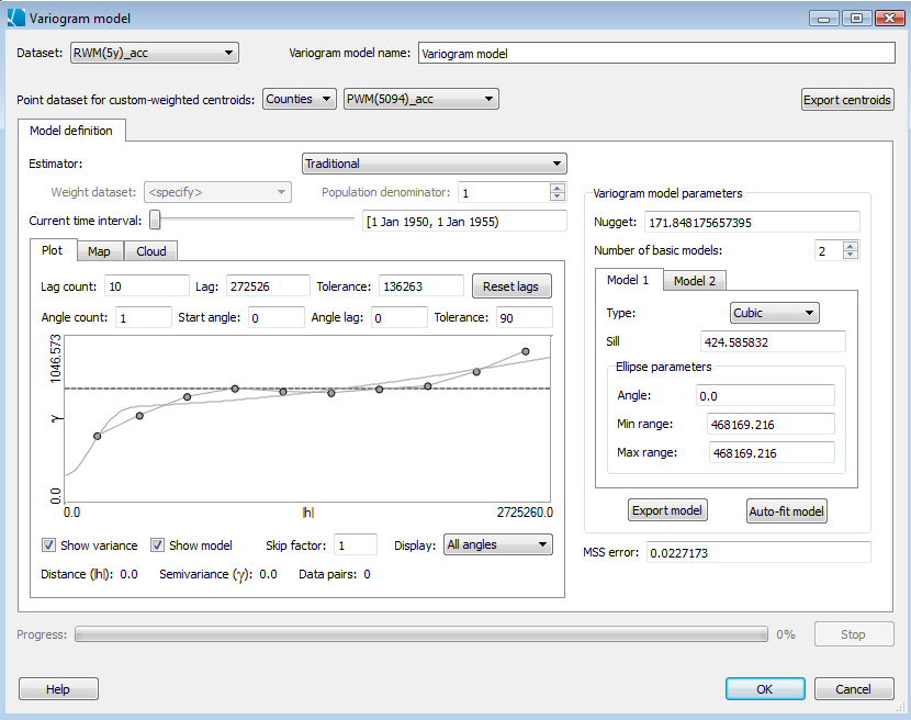
Dataset: Specify the dataset on which to perform kriging.  The user will not be able to create a variogram model if the values are all the same, or the associated locations all coincide.

Variogram model name: Specify the name of the variogram model.

Point dataset for custom-weighted centroids:  When kriging with polygons, the center-of-mass centroids are used when calculating distances between the polygons.  This parameter allows the user to use centroids based on weighted locations such as population centers.  For example, if the source geography is U.S. states, you might create population-weighted centroids for the states by specifying a U.S. county geography and a population dataset for the counties.  SpaceStat would calculate the population-weighted average of the county locations in each state.  Note that the purpose of this parameter is not simply to specify an alternative centroid geography.  If the user wants to examine the weighted centroid that is created, clicking the Export-centroids button will add the weighted centroid geography to your project.

Estimator:  The variogram estimator determines how the data pairs are used to create the variogram plot.  The traditional estimator uses the square of the difference between the data pair values.  The standardized estimator is the same but normalizes by the variance of the data.  The residuals, weighted and Poisson estimators all use a secondary dataset to modify the value associated with each data pair:  the residuals estimator first subtracts from each value of the data pair the corresponding mean dataset value before subtracting the values and squaring.  The weighted estimator multiples the squared differences by the associated weight in the specified weight dataset, and the Poisson estimator multiplies by a weight calculated from the specified population dataset and subtracts from the squared difference a population-weighted mean.  A more complete description is here.

Variogram model parameters

Here you can specify the settings for the variogram model and override settings for the model that's automatically created when the dialog is opened.  The nugget effect and the number of basic variogram models which comprise the full model are specified at the top.  For each basic model a type can be specified (spherical, exponential, Gaussian, cubic and power) and the basic model's sill.  You can also set the minimum and maximum range for the model and the orientation of the model if the ranges are different.  Note that if you choose to use a power model in your variogram you won't be able to conduct simple kriging which disallows this model type.  An XML description of the model can be exported by clicking on the Export Model button, and if you want to have SpaceStat auto-fit a model to your date click on the Auto-fit button.  This will bring up a dialog letting you specify the types of models SpaceStat uses when auto-fitting.  At the bottom is an indication of the mean sum-of-squares error between the experimental variogram and the current variogram model.

Plot tab

The variogram plot displays the experimental variogram based on the dataset's values and associated locations, and the current variogram model defined by the model settings.  The lag, lag count and tolerance fields define how the data pairs are binned by distance to create the experimental variogram's points.  By default (and when the Reset Lags button is clicked) the data pairs are grouped into 10 distance bins (the lag count).  The default distance lag is the geography's maximum radius (the half-diagonal of the bounding rectangle) divided by 10 and the tolerance is half the lag distance. If the tolerance is greater than the lag data pairs will be included in multiple distance bins.  Similarly, the data pairs can be segregated based on their directional relationships.  If the angle count is 2 then by default the data pairs are grouped into those falling within a 90-degree arc oriented to the right (the x-axis is 0 degrees) and those in a 90-degree arc oriented straight up.  The angle tolerance is half the angle lag by default.  Choosing more than one angle allows the variogram model to describe anisotropic trends in the data.  Finally, the skip factor allows for sub-sampling the data in cases where there are so many data pairs that model fitting is unacceptably slow.

Map tab

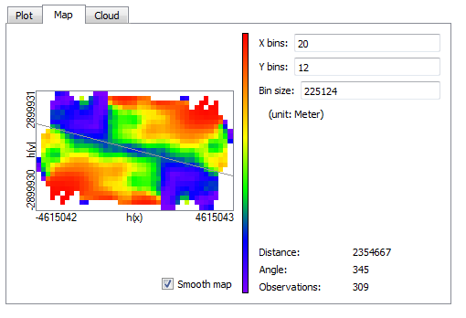
The variogram map is a useful tool for detecting anisotropic trends in your data.  Each block in the map represents data pairs whose relative directional relationship matches the direction between the block and the center of the map.  The color of the block indicates the similarity in data values between the data pairs in the block (purple and blue indicate similarity; red indicates disimilarity).  If there is meaningful anisotropy the map will show linear striping along some direction.  Moving your cursor in the map you can align the orientation line along the direction of least color change to determine the major axis of anisotropy, and use this angle as one of the start angles in the variogram plot.  The number of horizontal and vertical bins and bin size can also be specified.  This is analagous to the lag count and lag size in the plot tab.

Cloud tab

The variogram cloud is a tool for viewing the data pairs making up the experimental variogram model.  The default, frequency-raster mode bins the pairs into blocks whose pixel dimensions can be changed at the bottom right.  Alternatively you can have each data pair drawn on the map.  This mode is slower, but allows you to select outlier data pairs individually so you can exclude them in the calculation of the variogram model.  After selecting outliers right-click to bring up a context menu with appropriate options.

For an example of an analysis using the variogram model dialog, try the Variography tutorial.