Spatial Regression Results

Data View Results

All three forms of spatial regression will produce three datasets: the estimated mean, the standard error of the mean, and the residuals.  These datasets will be collected in a folder under the dependent dataset in the Data View.  This folder will have the name you specified in the Output folder name on the Regression settings tab.       

Log View Results

The type of spatial regression determines which set of results appear in the Log View.  All three types will list the parameters used in the method, which is the same information displayed in the Rum method tab.  The log will also report the datasets used in the model.  Then the log will report various model results for each time valid time interval.  

Ordinary Least Squares

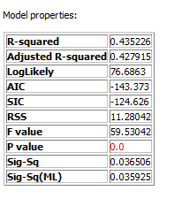
If you ran the ordinary least squares model, the first entry will be a table of model properties which will demonstrate various measures of overall model fit.  

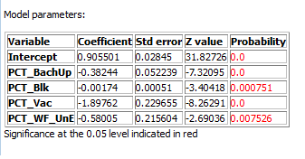
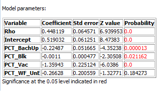
Next, the log will report a table of model parameters, including the coefficient, the standard error, the z-value and the p-value.  P-values which are significant at the alpha .05 level will be highlighted in red.  

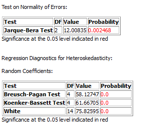
The next two tables in the log present tests for some of the assumptions of linear regression: normality and constant variance of the error terms.  The normality of the errors is assessed by the Jarque-Bera test, where a significant p-value suggests the presence of non-normality.

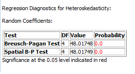
Three tests are given to assess heteroskedasticity, or non-constant variance.  These are the Breusch-Pagan test, the Koenker-Bassett test, and the White test.  Again, a significant p-value suggests the presence of non-constant variance.  

The final table for the OLS model present diagnostics for spatial dependence.  These tests use the spatial weight set given in the Regression setttings tab and assess whether the model might improve with the introduction of a spatial component.

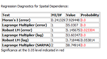
These tests are described in the section on diagnostics.  

Spatial Lag and Spatial Error

Both spatial lag and spatial error models will present a model properties table, but with less assessments than their OLS counterparts.

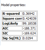
The model parameters table will be similar to the OLS table except the lag model will have an estimate of the rho coefficient (shown below) and the error model will have an estimate of the lambda coefficient (not shown).

Both lag and error models will use the Breusch-Pagan test as well as the Spatial B-P test to assess heteroskedasticity.

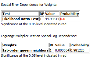
The next test is a likelihood ratio test for the model in question, either spatial lag or spatial error.  The difference in the calculated log-likelihood between the given model and the OLS version of the model is used as the statistic.  

The final test is the Lagrange multiplier test for spatial dependence.  This test takes the given model and examines spatial tendencies towards the alternate model.  In the table pictured below, we see the likelihood ratio test for the spatial error model and thus the Lagrange Multiplier test on spatial lag dependence.  

Again, these tests are discussed in further detail on the diagnostics page.