Perform Mixed Model Regression

Here we describe the settings that need to be specified to run the method. Open the project and go to Methods -> Regression -> Mixed model regression.  There are two panels.

Regression Models Panel

1. Select the geography corresponding to the lower level observations. Under the "Regression model" listbox a list of the names of saved regression models will be displayed. Select one of these - in the "Model  definition" window the details of each the listed models are given. If there are models listed click on the "Modify" button - if the list is empty click on the "Create" button.

   

2. You are now in the dialog entitled "Define mixed model".

   

   At the top is the model name which may be edited to your liking. Below that is a dropdown for the dependent variable. Select a dependent variable (or dataset).

   Next is a dropdown entitled "Upper level selection method" - there are two choices here: "Subject field" or "Upper level geography". In SpaceStat you can sort lower level data either by subject field or higher level geography. The subject field must be an integer that labels which of the upper level units each of the lower level observations belongs to. If you wish to sort the lower level data by a higher level geography then this is done automatically in SpaceStat.  All you have to do is specify the Upper level geography name.

   Choosing either "Subject field" or "Upper level geography" will enable either the "Subject field" or "Upper level geography" dropdowns that are next. Choose the subject field if there is one with your data, or if a higher level geography is included in the project pick the appropriate one. Please note that sensible choices for the upper level units must be made.  The maximum likelihood calculation will not converge otherwise.

   Next is the selection of independent variables which operates in the same way as for a-spatial, GWR and spatial regression models.  You will see a non-editable list of datasets remaining in the lower level geography. You can highlight one of these and click on the "Add linear term" or "Add squared term" buttons and to create your list of predictors. To create an interaction term select on dataset, hold down "Ctrl" key and select another dataset and click the "Add interaction term" button.  The "Linear terms", "Squared terms" and "Interaction terms" lists will display all terms currently in the model. These lists allow the user to remove existing terms by right-clicking and selecting "Remove". If a term is categorical then selecting it will enable the "Reference value" selection dropdown and the "Parameterization type" radio buttons. These are discussed in the help section on a-spatial regression.

   At the bottom is a box entitled "Term status- fixed or random". As regression terms are added to the model they are also added to this window. To the left of each term is a checkbox. Checking the box for a particular term will make that term "fixed" so that the regression coefficients will not be allowed to vary across the upper level units. Therefore the coefficients will be the same across the entire geography. Setting the box to unchecked will make that term "random" so its coefficients will be allowed to vary across the upper level geography units with a variance to be determined by maximum likelihood.  Always at the top of this list is the "Fix intercept" box. Again leaving this unchecked will allow the constant regression term (the intercept) to vary across upper level units. As a rule of thumb this is the first item to be left random in analyzing and exploring different mixed models. Usually the variance in the intercept is most often found to be significant.

   Note that at least one of the regression terms must be random (unchecked) for the model to be run. Otherwise one may just as well use aspatial regression. If there are no random terms a warning dialog appears when the user tries to run the model.

   At this point the OK button should be enabled and on clicking OK the regression model is created. The "Model definition" window displays the details of the current regression model. Next is the Regression Settings tab which is concerned mainly with computational details.

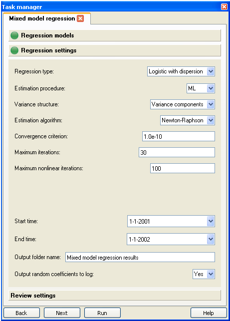
Regression settings tab

1. Regression type:  Default = Linear  

   You will need to inspect this setting.

   At the top is the regression type dropdown - this refers to linear, logistic or Poisson. The logistic and Poisson types can also be run with a dispersion parameter. Logistic mixed model regression requires the dependent variable to take values of 1 or 0.

2. Estimation procedure:  Default = ML  

   There are two likelihood based approaches: ML refers to the maximum likelihood approach while REML refers to the restricted maximum likelihood approach. The REML approach, although the default in most mixed model software, can take much longer than ML if the number of upper level units is large. Consequently we set the default to ML.  In cases where the REML approach is too slow under the Newton-Raphson estimation algorithm the user is recommended to set the estimation algorithm to EM.

3. Variance structure:  Default = Variance components

   This refers to the type of correlations expected between the random coefficients in the model. The output for the variances and covariances of the random coefficients is shown in the "Covariance Parameter Estimates" table in the Log view along with standard errors and p-values. There are two choices here (1) Variance components and (2) Unstructured. The default setting (Variance components) assumes that the variations of each of the random coefficients across the upper level units are uncorrelated with variations in the other random coefficients.

   The more general "Unstructured" setting assumes that there may be correlations between the variations of the regression coefficients across geographical units. The sign of an off-diagonal unstructured covariance parameter indicates whether regions with a positive value of one random regression coefficient are going to have a corresponding positive or negative value in another random regression coefficient. One can also see this reflected in a scatter-plot of the two sets of estimated random coefficients that are listed in the data view under the upper level geography. If the regression is run using the Variance components setting the scatter-plot will display no (or very little) correlation.

   The default Variance components setting should always be used first to test for vanishingly small variances in any of the random regression coefficients.  Such random coefficients should be set to "fixed" and the model run again. To do this the user should go back to the "Regression models" tab, select the regression model, click on the Modify button to open up the regression model dialog and check the checkbox next to the miscreant regression term in the "Term status- fixed or random" window.

   Once the random coefficients in the model are all found to have non-vanishing variances the user can safely explore correlations between the random coefficients using the "Unstructured" setting.

4. Estimation algorithm:  Default = Newton-Raphson.

   The two choices are (1) Newton-Raphson and (2) EM. The default Newton-Raphson approach uses a trust-region optimization approach to find the values of the random coefficients for which the likelihood is maximized using first and second derivatives of the log-likelihood. The EM approach uses an older but slower estimation-maximization algorithm. This setting is advised for REML estimation when there are a large number of upper level units and the user is carrying out exploratory analysis. It is also expected to converge under more general circumstances than the Newton-Raphson approach. However the default Newton-Raphson converges much faster. The user is encouraged to try both algorithms if time permits. The Log view displays the log-likelihood at each iteration.

   In either case the standard errors of the random coefficients are found from the Hessian obtained as the second derivative of the log-likelihood (either for ML or REML).

5. Convergence criterion: Default = E-10

   This refers to the point at which the maximum likelihood iteration procedure is judged to have converged. The number refers to the fractional change in log-likelihood at which the iterations will stop. The user can vary this setting to assess the convergence properties of the model.

6. Maximum iterations: Default = 30

   For linear regression this gives the maximum number of iterations that are allowed to attain convergence. For logistic and Poisson regression two such dropdowns appear because a double set of nested iteration procedures is used. The user can increase the maximum number of iterations if necessary to achieve convergence.

7. &

8. Start and End times:

   You will need to inspect this setting.

   The dates and times of the datasets in the model at which the regression analysis is to begin and end. In SpaceStat the number of time intervals can be large so analyses can take a long time. If the user is unfamiliar with the spacing of the time intervals in the project they can use the time plot feature or animate a map of the data. The user is advised to pick short intervals to run the method as a first step, especially if there are a lot of time intervals.

9. Output folder name: Default = "Mixed model regression results"

   This folder appears in the data view under the dependent variable dataset. The lower level datasets for the predicted means, residuals and standard errors are in this folder.

10. Output random coefficients to log: Default = No

    Choose "Yes"  if you want to see the estimates for the random coefficients in each of the upper units printed in the log view along with standard errors and p-values. This can take a lot of space in the log view but is the only way to see these estimates if the "Subject field" option is chosen in the regression model dialog.

Review settings

The review settings panel allows you to see all the setting used and may alert you to a parameter that has not been filled in correctly.  If everything is correct, click the Run button to run the method.