Implementation of the Back-Transform in Kriging

In presence of strongly positively skewed datasets, it is common to conduct kriging on the logtransformed values (lognormal kriging) or normal score transformed values (multiGaussian kriging). These transforms need to be done outside the kriging method since variograms are computed on the transformed values. Yet, the back-transform should be performed within the kriging method.

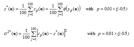
The back-transform equation is similar for both types of kriging. The kriging estimate and kriging variance of the original variable Z are estimated using the following empirical expressions:

where yp(u) are p-quantiles of the standard normal distribution (mean=kriging estimate, variance=simple kriging variance). The function f is: exp(.) for the natural lognormal transform, 10^ for log10 transforms,  and normal score back-transform for multiGaussian kriging.

There are instances where the back-transform does not make any sense, for example for Poisson kriging.

NORMAL SCORE BACK TRANSFORM

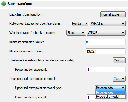
You will need to input the reference dataset whose distribution (i.e. histogram) needs to be reproduced. This would generally be the same dataset (and an optional weight set) entered for the input geography, but you have the flexibility to specify another dataset if you want. The distribution of the dataset is the necessary parameter, and so any geography could be specified here.

You will also need to provide the minimum and maximum values (zmin and zmax) for the back-transformed normal scores. By default, this would be the minimum and maximum of the dataset specified at the previous step.

If the maximum probability computed for the reference dataset is larger than the maximum value supplied, the default behavior for SpaceStat is to give that probability the maximum value specified.  Alternatively, you may employ the use of an upper tail extrapolation model. Two models are allowed: power model (with w parameter ≤ 1) and hyperbolic model (with w parameter ≥ 1). The default selection is a linear model (e.g. power model with w = 1)

Similarly, if the minimum probability computed is smaller than the minimum observation supplied, a lower tail extrapolation model may be specified. Only the power model (with w parameter ≥ 1) is allowed.  The default selection is a linear model (e.g. power model with w = 1).  These models are explained in great detail on pages 280-281 of Pierre Gooaverts' book.