Types of Kriging
The second panel of the kriging method is where users choose the type of kriging to perform. The options available change depending on whether or not there is secondary information available.
The panel also holds options for estimating spatial components (also known as factorial kriging) and employing a population adjustment method (Poisson kriging). If you choose to use the Poisson population adjustment method, you will have select the population dataset and the population denominator.
The input required from the user varies with each type:
|
Kriging Type |
User Input |
|
Simple kriging |
global mean |
|
Ordinary kriging |
-- |
|
Kriging with a trend |
trend components (X, Y, X2, Y2, XY) |
|
Factorial kriging |
-- |
|
Simple kriging with local means (kriging of residuals) |
local mean dataset, residuals variogram model |
|
Kriging with external drifts |
up to three drift dataset |
|
Poisson kriging |
population dataset and population denominator, poisson variogram model |
Implementation details for kriging
Let u0 be the prediction unit: point or polygon centroid.
1. Simple Kriging
The following kriging system is used:
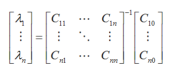
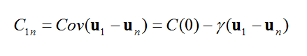
C1n is the ”data-to-data” covariance between locations u1 and un. It is computed as:
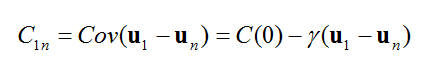
where C(0) is the sill of the semivariogram model, and g(u1 - un) is the value taken by the variogram model for the vector joining u1 and un. A similar expression is used for the ”data-to-unknown” covariance term C10.
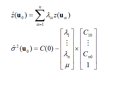
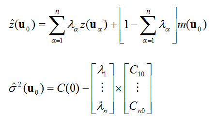
The vector of solutions (i.e. kriging weights) will be used to compute the kriging estimate and kriging variance datasets, computed as:

where n is the number of observations found in the search window, and m is the ”global mean” parameter.
2. Ordinary Kriging
The following kriging system is used:
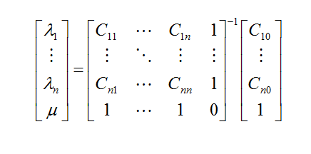
where m is the Lagrange parameter, and C1n is the covariance between locations u1 and un. It is computed as:
where C(0) is the sill of the semivariogram model, and g(u1 - un) is the value taken by the variogram model for the vector joining u1 and un. If the semivariogram has no sill (i.e. power model), the sill C(0) is replaced by a pseudo-sill A which is a large positive value such as A > g(h) for all h (PG book, page 135).
The vector of solutions (i.e. kriging weights) will be used to compute the kriging estimate and kriging variance datasets:
If the "Output trend coefficients" option is selected, a third output dataset (trend component) will be computed as:
where the kriging weights are computed as:
3. Kriging with a Trend
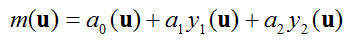
This type of kriging allows the user to select the number K of trend components, or trend functions fk. For example, if the boxes X and Y are checked, the trend model is:
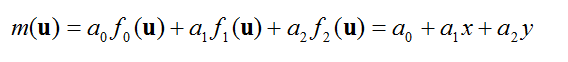
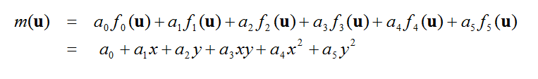
where x and y are the x-coordinate and y-coordinate of location u = (x,y). The function f0() is 1 by default, and other trend functions fk() k = 1,...,K are selected by the user. If the user checks all the boxes, the following quadratic model is selected:
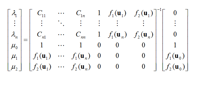
For example, if K=2, then the following kriging system is used:
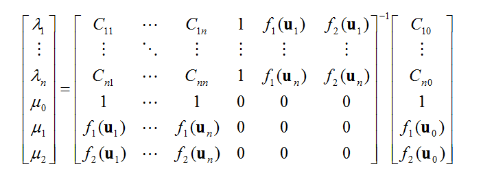
There are as many Lagrange parameters m as constraints in the system of equations. Note that the ordinary kriging system is just the particular case K=0.
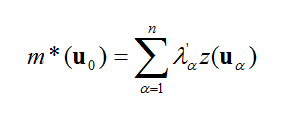
The vector of solutions (i.e. kriging weights) will be used to compute the kriging estimate and kriging variance datasets:

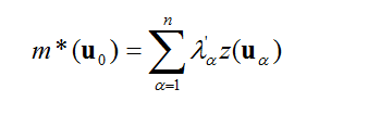
If the "Output trend coefficients" option is selected, (K+1) output datasets (trend component + K trend coefficients) will be created. First the trend component will be computed as:
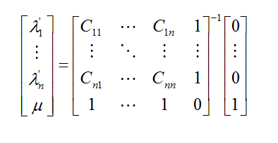
where the kriging weights are computed as:
Second, each of the trend coefficients ak for k>0 will be estimated as:
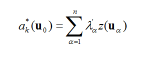
The kriging weights are computed as:

where  if k’ = k and 0 otherwise.
4. Factorial kriging
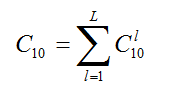
In factorial kriging, spatial components corresponding to the different basic semivariogram models are interpolated. For example, if the semivariogram model consists of L basic models (i.e. L=2 for one nugget effect and one spherical model), the ordinary kriging estimate can be decomposed as:
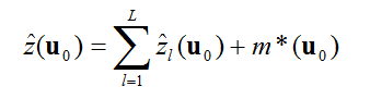
The kriging estimate, kriging variance and the trend component m*(u0)
will be computed according to the equations described for ordinary kriging).
In addition, each of the L spatial components  is
estimated as:
is
estimated as:
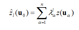
The kriging weights are computed as:
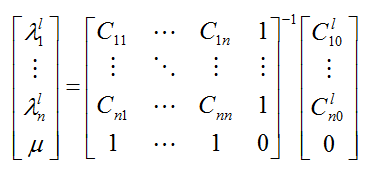
is the covariance between locations u1 and u0 for the lth basic model. The following relation is satisfied:
5. Simple Kriging with Local Means
The following simple kriging system is used:

The vector of solutions (i.e. kriging weights) will be used to compute the kriging estimate and kriging variance dataset:
where n is the number of observations found in the search window, and m(u0) is the "local mean" dataset.
6. Kriging with External Drifts
The user may selects K "drift" datasets: yk(u), k=1, ... ,K. These datasets are used to model the trend of the variable z to be interpolated. For example, if two drift datasets are selected, the trend model is:
This formulation is similar to the trend model used for kriging with a trend, where f0()=1 by default, and the other trend functions fk()=yk(). The same equations can be used to compute:
- the kriging estimate and kriging variance.
- (K+1) output datasets (trend component + K trend coefficients) if the "Output trend coefficients" option is selected.
7. Poisson Kriging
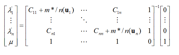
The following kriging system is used:
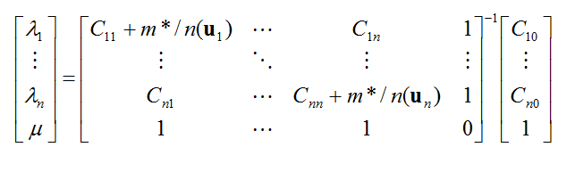
The only difference between this system and the ordinary kriging system is the diagonal of the matrix where an error variance term, m*/n(ui), is added to each of the covariance term Cii. m* is the population-weighted mean of the rate dataset, and n(ui) is the population at that location.
The vector of solutions (i.e. kriging weights) will be used to compute the kriging estimate and kriging variance datasets.
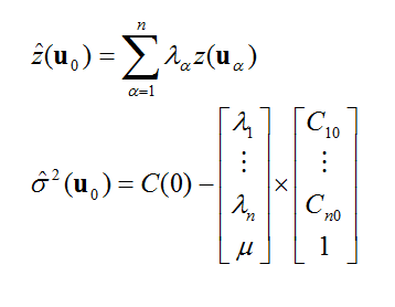
If the "Output trend coefficients" option is selected, a third output dataset (trend component) is computed as:
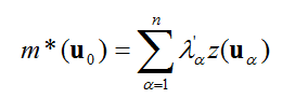
where the kriging weights are computed as: